The life changing magic of tidying text files

Posted in RStats on rstats, datatable, purrr

Bringing order to irregularly structured open data CSV files - with R, of course

Our team have been doing some work with the Scotland Census 2022 data. There are several ways to download the information - you can click around on maps or use a table builder to focus on specifics, or there is a large zip download that provides all the data in CSV format. You end up with 71 files, with around 46K rows and a variable number of columns.

• The first 3 rows of each file contain generic information about the dataset and can be discarded for analysis. Because these are of varying widths, various file readers may trip up when reading them in. data.table suggests using fill = TRUE when using fread, but that causes immediate failure in some cases.
• The last 8 rows contain text that can also be discarded. (In truth, these rows never got read in because the single column threw fread, which was a blessing in disguise)
• Once these rows have been discarded, many files have headers in multiple rows which need to be extracted, combined, and the added back as column headers.
• Need to account for having between 0-5 rows of column headers, with some blank rows in between, usually around line 4 or 5
• Some files have extra delimiters in the first 3 rows

Obviously, for one or two files on an ad-hoc basis, you can get around this by hand, or other nefarious means. Doing it programatically is another issue. It’s just the right kind of problem - tricky enough so that you can’t stop thinking about it, and easy enough that you can actually achieve something.

My initial approach involved 2 reads per file - I read the file in and saved as a temp file, then used scan on the temp file to find the first Output Area code in the first column - this is the first row of data. Then I created some vectors of indices for where the data began, and where I thought the actual first line of header rows were, after skipping the first 3 rows.

I tried using {vroom}. For this to work I needed to provide a skip value and set col_names to FALSE. There was no way to get an accurate skip value without doing a prior read or scan.

Then I decided to go back to fread and not skip anything, set header to FALSE, and perform only one read. data.table was smart enough to strip out the first three rows anyway, so I was left with the multiple rows containing the column headers right at the start of the table.

I skimmed those off using grep to find the first output area, and subtracting 1 to get the correct number of header rows

# find the row with the start_target value, and retrieve all the rows above it
headers <- int_dt[,head(.SD,grep(start_target,V1) - 1L)]

Using tail on the data, with a negative index to account for the number of header rows, gave me the actual data. I just used dim of the headers data.table to get the number of rows, to save performing another grep

# remove the first n header rows - the rest of the rows are the data we need to process
  int_dt <- int_dt[,tail(.SD, -dim(headers)[1])]

After that, it was a matter of combining the headers rows and collapsing them into a character vector and setting those as the column names. Then I pivoted the data into long format, copied the value column, replaced hyphens with NA, and coerced to numeric. I added in options to write the file out, or to print, or to return it in case further processing was required.

Here is how I used data.table’s set operation to remove instances of 2 or more underscores in the variable column. Note the use of .I to return an integer vector of rows to update

# replace any multiple underscores in variable column
  col_name <- "variable"
  rows_to_change <- out_dt[variable %like% "_{2,}",.I]
  set(out_dt, i = rows_to_change, j = col_name,
     value =  stri_replace_all_regex(out_dt[[col_name]][rows_to_change],
     pattern = "_{2,}",
     replacement = ""))

As this is data at a very small geographic level, for all of Scotland, we don’t want to be writing these out to a CSV file (although, my function saves them as .TSV by default). I used the arrow package to write them to parquet. And, used duckdb to create a duckdb database.

The code for all this is on my github here tidy_scotland_census

Further developments would be to filter this for specific areas - I am only really interested in Highland and Argyll and Bute- however I’ve left this for now so the code should be of use to anyone who wants to use it.

There is some example code of how to use the function with purrr to write the files, or view the outputs in tidy format. You could also stick them in a nested list (1.7 GB), but my immediate reaction to doing that is to try and get it straight back out again. I do recommend using purrr’s safely function for this sort of thing.

Having sorted out the approach, I spent some time trying to make things a bit faster. Using gsub was slowing things down, so I replaced that with some stringi. Coercing to numeric also took some time, but even using a set approach in data.table did not speed things up. That was because I was creating a vector of indices to pass to the set syntax (for j in cols), and it was pretty slow operation. Switching back to subsetting and using let to update by reference was much faster. I’m not sure this should generally be the case, but I tried both methods with several files. I used the profvis package to figure out where the bottlenecks were, and it was very handy to confirm my original approach was faster.

In general, this whole approach can be used elsewhere, not just for these census files.

Although your CSV’s may be irregular, there is a way to deal with them and get your data into a useful shape.

My top tips:

• don’t panic : look for some common ground, even if the number of rows/ columns, headers varies by file. In this case, it was seeing the first row of actual data began with the same value, and that it would occur within the first ten rows.
• don’t try and eat the elephant. It’s easy to chuck a function into map or another purrr function and apply it en-masse. But it’s easier to get things working for one step at a time on the same file, and then branch out to others.
• use purrr safely. See the code for some functions to get data back out of the resulting list
• base string functions are very useful, and overlooked

Addendum: coming back to this today, having tidied a file up in Power Query, I realised everything could be much easier. Power Query discarded the first few rows of text, and so filtering for blanks in the second column gave me the header rows. I was able to transpose those and combine them, then transpose back to give me one row of headers.

I isolated the non header rows as a seperate table, read the data in again minus those rows, combined both tables and unpivoted everything but the first column.

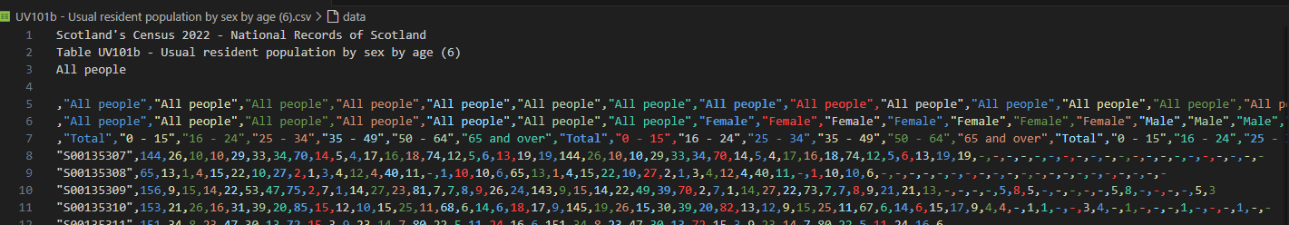
The reason I didn’t spot this earlier is that you get a much better view of the data in Power Query than in the quarter pane of RStudio. Similarly, I wasn’t getting the same sense of the data structure when viewing it in VS Code either. (The header image for this post shows how the first few lines of one file looked in VS Code).

I was able to do the same steps using R to isolate the header rows. A quick fsetdiff between the original data and the headers gave me the data. Then I performed the same steps as in my original approach to join the rows in the headers together and set them as the column names in the main dataset. This approach was slightly slower for the first file, but definitely quicker for the largest file in the set, which returns over 20M rows.

Now, having cracked the transformation for one file in Power Query, I have to figure out how to do them all. But that’s for another time.